A detailed walkthrough of the development, intended for anyone setting out to build something similar 🤗.
Generals.io1 is a real-time strategy game with a simple premise. You start as a single crown on a grid, grow an army, spread across the map, and try to capture your opponent's general before they capture yours. The rules take about a minute to learn, but much like Go, that small rulebook unfolds into enormous complexity: games grow into board-spanning fights where a small early advantage can compound for hundreds of turns.
That depth has kept a community around for years — thousands of players, active 1v1 and team formats, regular tournaments, and bots going back nearly a decade.
the game The rules, in about a minute ▶
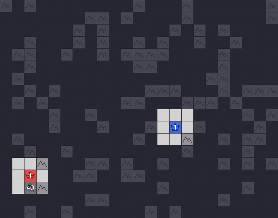
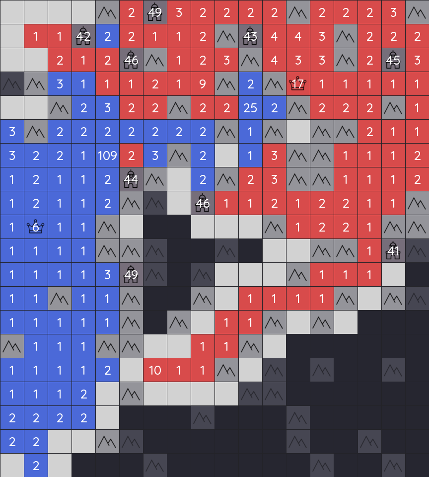
The game is played on a grid of square cells. Most are plains — empty, passable tiles; moving onto a neutral plain simply makes it yours. Scattered among them are mountains, which are impassable and permanent, and neutral castles, fortified tiles that start with a garrison of 40–49 army. Each player begins on a single general — the crown you have to protect. Lose it and you lose the game.
The game advances in discrete turns, and on each turn you make one move or pass. A move pushes the army stacked on one of your cells into an adjacent cell — up, down, left, or right — carrying either all but one unit or half the stack. You always leave at least one behind. Moving onto another cell you already own just merges the two stacks; moving onto a neutral plain claims it.
The main resource is army, and it can grow in two ways. First, your general and every castle you hold each produce one unit every other turn, so holding more castles means a faster-growing economy. Second, every 50 turns every tile you own gains one unit at once. Captured plains produce nothing between those 50-turn ticks, so most of your army comes from generals and castles.
Move onto a cell someone else owns and the two army counts collide: they subtract, and you take the cell only if you arrive with strictly more, keeping the difference. A neutral castle works the same way against its garrison — 41 units to take a castle holding 40. Capture the enemy general and you win on the spot.
You do not see the whole board. Vision is limited to the cells you own and their immediate 8-cell neighborhood; everything else is hidden in fog. A scoreboard tells you roughly how much total land and army the enemy has, but not where that army is massing or where their general sits — you have to infer it, and they are inferring the same about you.
the game What makes the game interesting ▶
Generals.io looks simple but stays interesting and difficult for multiple reasons.
- Resource management. At its core it's a resource game: a growing army to spend, and constant long-term choices about how to distribute it — where to expand, which cities to take, which directions to commit an attack from.
- Huge action space, long games. Each move offers hundreds of legal actions, and a single game easily runs a thousand moves. That is hard both from a planning and strategy perspective and for credit assignment — tying the final win or loss back to the handful of moves that actually decided it.
- Fog of war. Most of the board is hidden, so the agent must continuously update its belief about enemy intent and army distribution — hard in itself. The fog also invites feints and gambles — marching deep into enemy territory without knowing whether you'll find their general or just lose the army you committed — and up close those turn into sharp, fast exchanges that reward precise movement. It's where the most fun moments happen.
Human.exe
Human.exe2 is a
strong bot that has beaten many players, including some with
hundreds or thousands of games. It is an impressive piece of
hand-engineering (created before the vibecoding era, wow): a strict
priority cascade of roughly thirty precomputed plans, a belief model
that tracks enemy armies through the fog, and classical optimizers
(prize-collecting Steiner trees, min-cost flow, a minimax for
short-range fights and capture/defend races). For years it was the
bot to beat.
It represents a particular philosophy: encode human knowledge, carefully, by hand. Which runs straight into one of the most quoted ideas in modern AI — Rich Sutton's bitter lesson3: in the long run, general methods that scale with computation tend to overtake systems built from hand-crafted human knowledge.
So there was an obvious bet to make. A learning agent, given
enough compute and the right training loop, should be
able to surpass even a bot as carefully built as
Human.exe — without being told a single
human rule. So building one became my master's thesis.
Round one was my master's thesis, built in two stages: supervised pretraining to imitate human play, then reinforcement learning to improve on it through self-play. The idea was to get an agent that plays at all, then push it further.
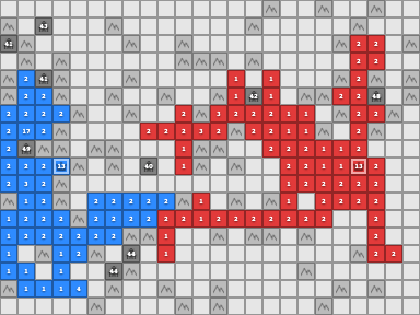
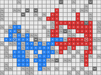
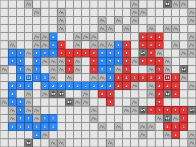
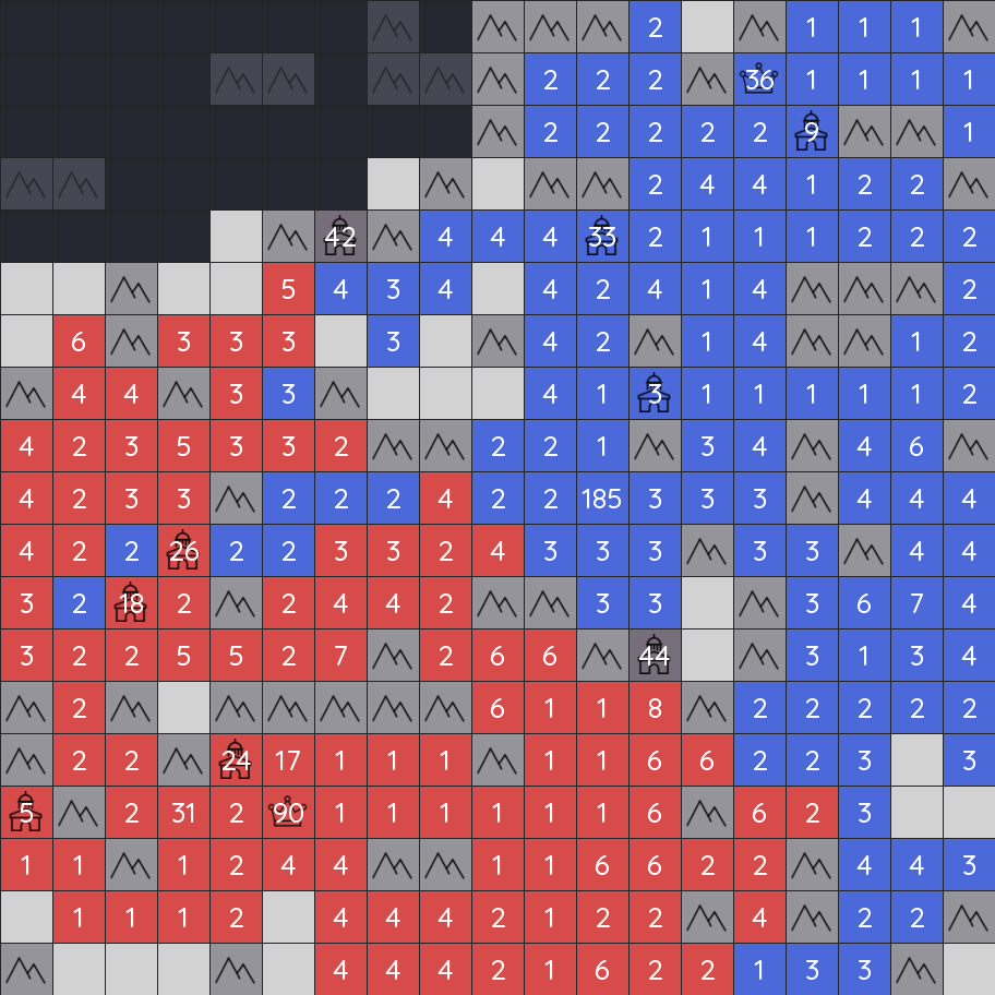
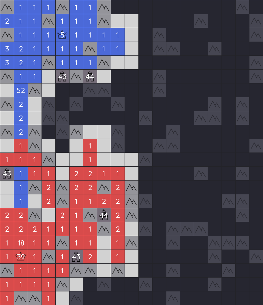
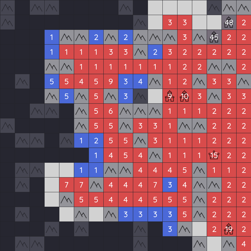
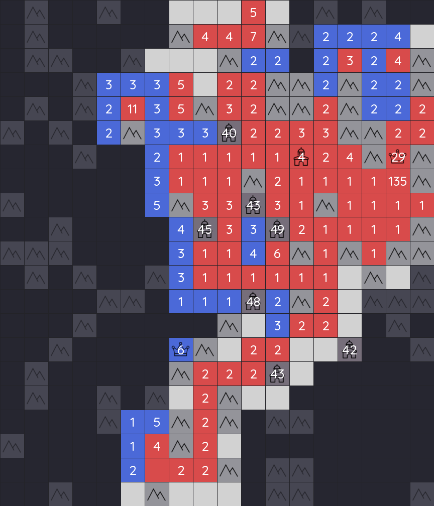
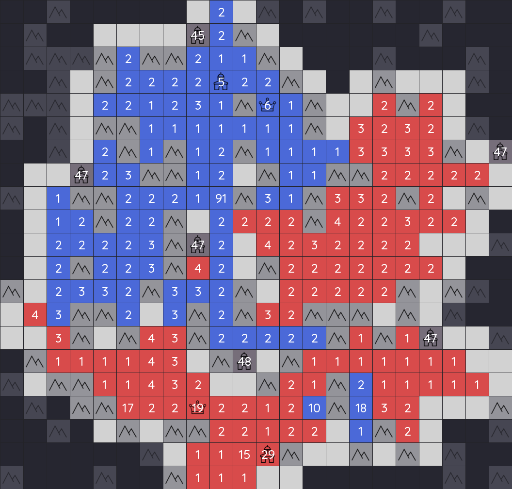
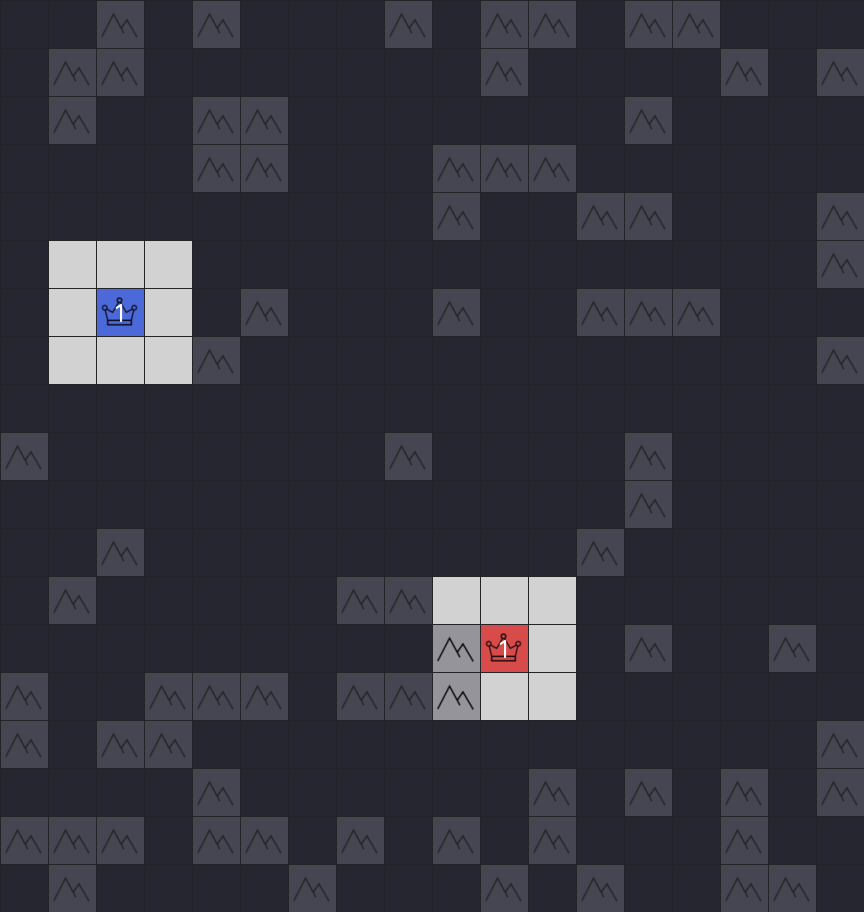
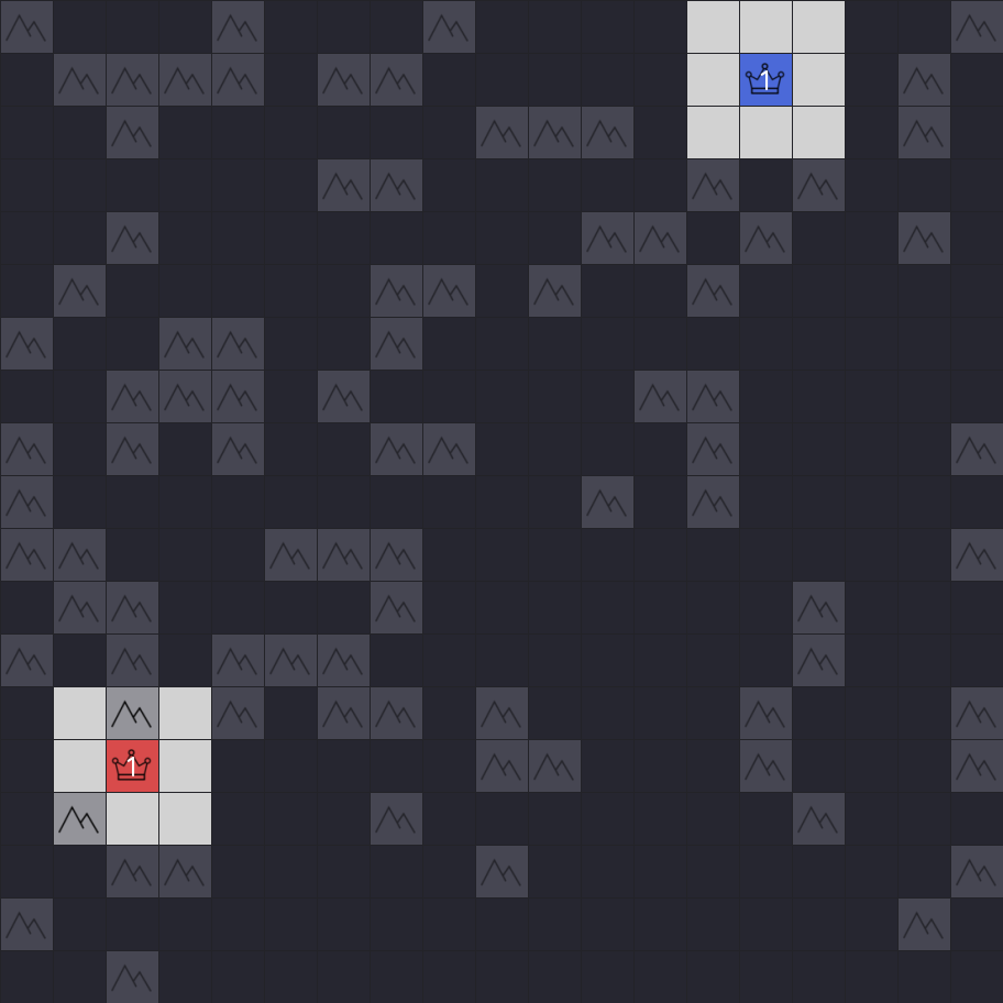
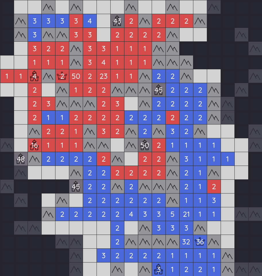
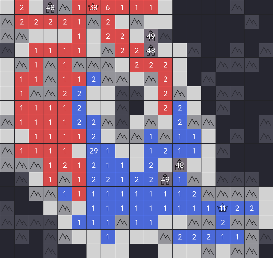
A few of the agent's games to set the scene. Swipe through the gallery.
Stage one: learning from humans
Dataset
Training an agent from scratch on a small compute budget is hard. At the start it moves at random, and on a full-size board it almost never captures the enemy general, so the win/loss signal it needs to learn from almost never appears. Supervised pretraining avoids this by starting from human play instead. Generals.io keeps match replays on its servers, and 347,000 of them were downloaded as the raw dataset; filtering then removed the degenerate games and kept only those involving strong players, leaving 16,320 games, about 9 million moves. The cleaned dataset is on 🤗 Hugging Face.
under the hood How the replays were cleaned ▶
The raw replays could not be used directly. They came from many different versions of the game, and many were matches where neither player tried to win — some lasting twenty thousand moves with both sides idle. These made up a large share of the data, and they break supervised pretraining: the objective only predicts the move that was played, not whether it was good. With the idle games left in, the most common action is to do nothing, so the pretrained agent learned to do nothing.
Two filters produced the final dataset. The first removed the degenerate games: only matches that finished within a reasonable number of turns, and where each player moved on at least 80% of their turns, were kept. This discards the idle replays that otherwise dominate the move distribution.
The second filtered by player strength, which trades quantity for quality — restricting to stronger players leaves fewer games. Sweeping the rating threshold showed that keeping games with a player rated at least 70 ⭐ gave the best result: 16,320 games, roughly 9M steps.
The observation fed to the network includes features from the game's history — what has been revealed, where the enemy was last seen, recent moves — so frames can't be shuffled independently. A custom dataloader loads each game step by step and reconstructs these history-augmented observations on the fly.
Network architecture
The network's input is the board encoded as a stack of feature planes — terrain, cell ownership, army counts, and the fog-of-war mask — together with memory planes that summarize the game so far: the last known positions of revealed generals and castles, which cells have been explored, which cells the opponent has seen, and the recent moves of both players. Under fog of war most of the board is hidden on any given frame, so these memory planes give the network a compact view of the history it would otherwise have to learn using memory modules such as an RNN.
Comment Why not learn the memory instead? ▶
Learning a memory mechanism from scratch (a recurrent state the network maintains on its own) is the more general approach. We were confident it isn't needed for very strong play, though: remembering a handful of hand-picked facts about the history is enough — and the project bears that out, with round two reaching superhuman play on only hand-crafted memory, no learned recurrent state.
It also saves a lot of compute. A recurrent memory has to be unrolled over the sequence during training, which makes each iteration much slower; precomputing a few memory planes keeps the training loop fast.
Still, learning the memory rather than hand-crafting it is the natural next step — it would very likely make the agent stronger still.
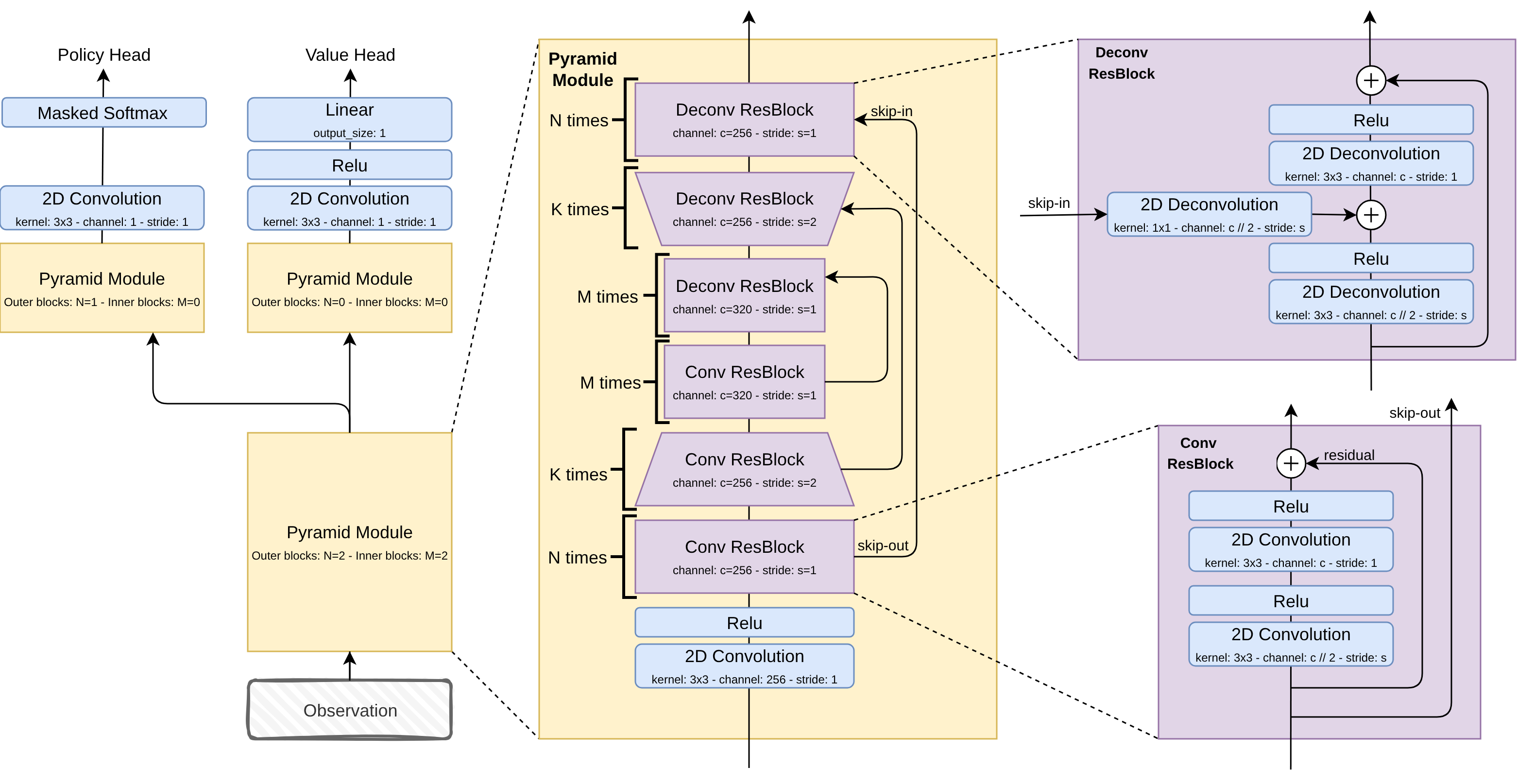
The architecture is U-Net style, taken from DeepNash4, which used it for Stratego. A convolutional U-Net torso turns the stacked observation into a board embedding that feeds two heads, one for the policy and one for the value; the implementation is on GitHub.
Training objective
The action space is defined per cell: for every cell the agent
can pass, or move all or half of its units in one of the four
directions — an H×W×9 grid of
possible moves. Pretraining optimizes both heads at once. The
policy head is trained by cross-entropy to predict the move the
human actually played at each step — this is the part that
matters for behavior cloning. The value head, trained to predict
which player eventually won the game, isn't needed to imitate
moves at all; it is trained because stage two is actor-critic, and a
critic warm-started on human play is a far better initialization
than a random one.
Trained this way, the pretrained network already played like a competent human — strong enough to reach roughly the top 150 players on the ladder, a 61 ⭐ rating. That was the starting point for stage two.
Stage two: reinforcement learning
Behavior cloning extracts what it can from human games, but it can only imitate — the policy never surpasses the players it learned from. Going further means producing new data rather than replaying old games, which is what reinforcement learning is for: the agent plays, keeps what works, and improves from its own results.
Training is self-play: the agent's opponents are frozen copies of earlier versions of itself — beat the snapshot, become the snapshot, repeat.
Simulator
Those games have to be played somewhere, so a custom Generals.io simulator was built. Because reinforcement learning is data-hungry, the environment is vectorized to run many games in parallel, and it exposes a gym-like interface, so the training code looks like any other RL setup.
The simulator ran on CPU, and that was the bottleneck rather than the GPU: training went only as fast as games could be produced. To get more out of each iteration, only the policy and value heads were fine-tuned while the U-Net torso stayed frozen; updating the whole network barely helped at this stage and was much slower.
The training objective
The agent is trained with PPO5, an actor-critic algorithm. It learns two things side by side: a policy (the actor) that picks the moves, and a value function (the critic) that estimates how well the agent can expect to do from a given state.
It plays, and for every move it compares how things actually turned out against what the critic expected. Moves that did better than expected get increased probability, moves that did worse get decreased probability. PPO adds one safeguard: a single update can't drift the new policy too far from the previous one, so the agent improves in small, safe steps.
under the hood PPO and GAE in detail ▶
Each update maximizes the clipped surrogate objective \(J(\theta)\):
Here \(\pi_\theta\) is the actor, the policy itself, and \(\pi_\theta(a_t \mid s_t)\) is the probability it assigns to action \(a_t\) in state \(s_t\). The ratio \(\rho_t\) is that probability under the new policy over the old one, so it measures how far the update has shifted a given action; clipping it caps how far a single update can stray from the policy that collected the data — a trust region of width \(\epsilon\) that keeps each step small.
The advantage \(\hat{A}_t\) is how much better or worse than expected a move turned out, where “expected” is the critic's value estimate \(V\). The simplest way to measure it looks one step ahead: take the reward \(r_t\) actually collected at step \(t\), add the critic's value of the state reached \(V(s_{t+1})\), discounted by \(\gamma\)?Discount factor γIt sets how much future reward counts: rewards add up as r₁ + γ r₂ + γ² r₃ + …, so γ < 1 makes distant reward worth less. At γ = 1 every step counts the same., and subtract the value of the state left behind \(V(s_t)\). That is the one-step temporal-difference (TD) error:
Nothing forces the estimate to stop at one step. It can use three real rewards before falling back on the critic, or run all the way to the end of the game and use no critic at all:
The further out the estimate looks, the less it leans on the critic: short ones have low variance but inherit the critic's bias, long ones are unbiased but noisy, since one move's effect gets buried under many random rewards.
GAE6 blends all of these \(n\)-step estimates into one. It collapses into an exponentially-weighted sum of the TD errors:
The dial \(\lambda\) slides between trusting the next step (\(\lambda \to 0\), the one-step TD error) and trusting the final result (\(\lambda \to 1\), the full-game return). Either way the advantage is only as good as the critic underneath it.
The full PPO objective adds two standard terms to the surrogate: an entropy bonus \(H(\pi_\theta)\) that keeps the policy from collapsing prematurely onto a narrow strategy, and a value-function loss that trains that critic, with \(\alpha\) and \(\beta\) weighting the two.
under the hood Why plain PPO self-play, not a dedicated equilibrium solver ▶
Under fog of war, 1v1 Generals.io is a two-player zero-sum game of imperfect information. The strategy you ultimately want is a Nash equilibrium: it is unexploitable, and because 1v1 Generals is symmetric, it secures at least a draw in expectation against any opponent. Dedicated solvers like CFR14 can compute one exactly, but they don't scale — in a game the size of Generals.io, an exact equilibrium is intractable. The practical alternative is to chase an approximate equilibrium with reinforcement learning, the idea behind methods like PSRO9 and NFSP12.
More recently, Magnetic Mirror Descent (MMD)10 was shown to converge provably to (quantal-response) equilibria in exactly these games. Its only addition over a plain policy gradient is a KL anchor to the previous policy — and PPO's clipping already enforces that same trust region. So for all practical purposes the policy gradient used here is MMD, which is why plain PPO self-play is enough.
The empirical case for staying simple keeps getting stronger. Rudolph et al.11, across more than 7,000 training runs, found that deep-RL methods built on fictitious play, double oracle, and CFR fail to outperform generic policy-gradient methods like PPO on imperfect-information games. So plain PPO self-play isn't a corner cut and hoped to hold — there is both theory and evidence that it is competitive with the heavier game-theoretic machinery.
The RL phase already improved on the behavior-cloning agent, but it always converged to a single style: extremely aggressive, mostly gathering army and attacking. Against humans this worked surprisingly well — it climbed from around the top 150 to the top 100 of the ladder — but players who knew how to defend and build a lasting advantage could beat it.
Stage three: patching a local optimum
That aggressive style wasn't the only thing the agent could have learned — it was a local optimum, and on the compute budget of round one, a hard one to escape. Aggression works well enough that the gradient keeps pointing back at it, and without enough exploration to find the slower, more positional lines, the agent never climbs out. One way out is more compute: explore wider and longer until the better optimum surfaces. The cheaper way is to patch the objective and nudge the agent out of the basin by hand. Round one took the cheaper route, with two patches on top of plain self-play: reward shaping and a poor man's fictitious play, each covered below.
Reward shaping
In plain self-play the reward is very sparse: just \(\pm 1\) at the end of the game. With \(\gamma = 1\)?Discount factor γIt sets how much future reward counts: rewards add up as r₁ + γ r₂ + γ² r₃ + …, so γ < 1 makes distant reward worth less. At γ = 1 every step counts the same. that means every action in a game gets the exact same credit, even though they didn't contribute equally — a winning game can still contain bad moves. Working out which actions actually deserve the credit is the famous credit assignment problem.
One way to help is to not give reward only at the end of the game, but after every action, based on how good that action seems. The risk is that hand-crafted reward functions often get exploited by the learning algorithm and don't yield the behavior you wanted. But one form of shaping avoids that — potential-based reward shaping7 (PBRS). It assigns a potential \(\phi(s)\) to every state, and on a move from \(s\) to \(s'\) it adds an extra reward equal to the change in potential:
So the original reward is augmented by the difference of potentials: move to a higher-potential state and the action gets rewarded more, move to a lower one and it gets penalized. In our case the potential is a weighted sum of log-ratios?Why a log ratio?It's symmetric around parity — twice the opponent's army reads as +1, half as −1. A raw ratio would be skewed: +2 versus −½. between the agent's and the opponent's land, army, and castle counts:
In plain terms, the potential \(\phi\) is high in states where the agent is materially ahead (more land, army, and castles than the opponent) and low when it's behind.
Potential-based shaping comes with a guarantee that ad-hoc reward bonuses don't: it leaves the set of optimal policies unchanged. The dense signal changes how fast the agent learns, not what it is ultimately trying to do.
under the hood How the shaping telescopes, and what it ends up rewarding ▶
An action's credit is its return — the discounted sum of rewards earned from that state onward. Writing \(s_0\) for the state where the action is taken (any state in the game, not just the opening) and \(s_T\) for the terminal one, the original return is
Shaping adds the change in potential at every step. Sum the shaped reward the same way and the potential terms telescope down to the two endpoints:
The original reward \(r_t\) is zero everywhere except the last step, where it is \(+1\) for a win or \(-1\) for a loss, so the first sum is just that terminal reward. Defining the potential to be \(0\) at terminal states makes the \(\gamma^T \phi(s_T)\) term vanish; with the undiscounted reward used here (\(\gamma = 1\)) the shaped return collapses to
The offset \(-\phi(s_0)\) depends only on \(s_0\), not on the action taken there, so it shifts the return of every continuation from that state by the same amount. It can't tip the balance between two moves, so the set of optimal policies is left exactly as it was.
What the offset does change is how large the signal is from each state. If \(\phi(s_0)\) is low (the agent is behind) and it still goes on to win, the return is \(1 - (\text{small}) \approx 1\), a strong reward for the action that escaped the low-potential state. If \(\phi(s_0)\) is already high, near \(1\), the same win is worth \(1 - 1 \approx 0\): the action barely contributes, since the game was effectively won already by the earlier moves that built the lead.
That guarantee is weaker in practice than it sounds: it describes the limit, not the finite-compute path, and runs with different \(c_1, c_2, c_3\) converged to visibly different players — one expands harder, another hoards army, another prioritizes castles. The improvement itself, though, was strong and consistent across all of them: every shaped variant beat the unshaped agent comfortably, expanding territory far more effectively and sometimes investing in capturing a castle — something the attack-everything version never did.
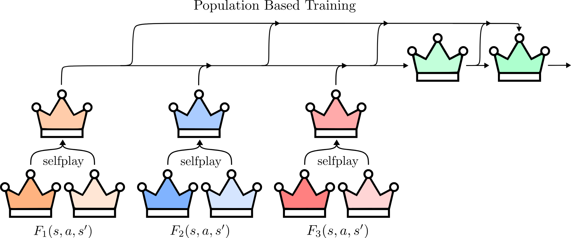
A poor man's fictitious play
Training only against the latest copy of itself, the agent can overfit to that single opponent and fall into non-transitive cycles rather than improving steadily. A pool of past versions instead pressures it toward play that is robust across opponents.
So the agent instead trains against a small pool of its own checkpoints. The pool is kept at three agents, each with its own style; every game is played against one of the three, drawn at random. Once the learner's win rate against the pool passes 60%, a fresh snapshot of it joins and the oldest agent drops out, and training continues against the updated pool. It is a poor man's fictitious play8: a handful of checkpoints rather than full neural fictitious self-play (NFSP)12, but enough to make it robust to more than one style of play. Round two drops it entirely, relying on MMD's convergence properties instead of a hand-built pool.
under the hood What “sampling an opponent” actually means ▶
“Each game's opponent is sampled at random” is a slight simplification. Experience is collected in fixed-length blocks: a rollout runs for 600 steps, split into chunks of 200, and a single opponent is drawn from the pool and held fixed across every parallel environment for the chunk before the next one is sampled.
So games lasting longer than 200 steps are played by multiple opponents. That does no harm — if anything it helps, exposing the learner to a wider mix of styles inside a single game, a cheap extra source of augmentation.
Where round one landed
Behavior cloning, then shaped self-play against the checkpoint pool, cleared the wall — a learning agent above the strongest hand-engineered bot, with no human rules anywhere in it.
Most of that climb was likely reward shaping alone, not the pool on top.
The Human.exe edge is real (95% CI 50.6–59.0%); round two
closes the gap to the very best humans.
After the thesis wrapped up, we counted it a success — but it still bothered me that round one couldn't be pushed any further. So I looked back and saw that its limits had a recurring shape. Supervised pretraining existed because a from-scratch agent on a slow simulator would almost never stumble into a win. Reward shaping existed because the true win/loss signal was too sparse to learn from on the samples available. Both were patches on the same deeper problem: the training loop couldn't generate enough experience, so ad-hoc tricks were used to squeeze the most out of what little there was.
So for round two I stopped bandaging symptoms and went after the sickness itself: the experience bottleneck. Rather than work around a starved training loop, the whole stack was rewritten in JAX to maximize simulator throughput and built on architectures that scale with data, so experience stopped being the constraint. With the bottleneck gone, the patches had nothing left to do, and every one of them went:
- No behavior cloning. The agent never sees a human game.
- No reward shaping. Sparse win/loss reward only.
- No population, no pool. A single policy, plain self-play.
What replaced the patches was speed and a few targeted choices: the JAX simulator at ~50M steps/s, a transformer policy, a parameter EMA at deployment, and advantage filtering. This agent reached #1 on the ladder and beat the top humans head-to-head. The sections below cover each piece in turn.
A simulator 10,000× faster
The first critical piece was rewriting the environment in JAX. Round one's simulator ran on CPU — 64 cores, 128 parallel games, roughly 3,500 steps per second, with the GPU mostly waiting for rollouts. Done right, a JAX rewrite moves the entire game onto the accelerator: board state lives in arrays, the rules become vectorized array operations, and tens of thousands of games step in lockstep as one program. On a single GPU, throughput went from ~3,500 steps per second to ~50 million — a four-orders-of-magnitude jump.
Samples that cheap change what's necessary. There's no need to bootstrap from human games when the agent can play billions of its own, and no need to densify the reward when the sparse win/loss signal arrives millions of times per run. The patches from round one didn't have to be carefully replaced — they simply had nothing left to patch.
under the hood Not just the env — everything is JAX ▶
The environment is only a third of it: the network and the entire training loop are written in JAX too, and that is the real unlock — end-to-end JIT. One training iteration — stepping tens of thousands of games, running the policy on their observations, computing advantages, taking the gradient step — compiles through XLA into a single program that lives on the GPU.
That eliminates the classic RL bottlenecks in one move. There is no Python in the hot loop, and no CPU↔GPU round-trips: in a conventional setup, observations and actions cross the bus every step and each side stalls waiting for the other. Compiled end to end, the data never leaves the device, and the compiler can fuse and overlap work across what used to be hard boundaries between “environment”, “inference”, and “update”.
For a concrete sense of how much that hot loop costs: an
early version already had the simulator and the network in
JAX, but still stepped the rollout from a plain Python
for loop — call the policy, pass the
actions to the environment, store the outputs, repeat. Each
step of that loop bounces back through the interpreter.
Folding it into a single jax.lax.scan, so the
whole rollout compiles into one program, was worth another
~10× in smaller settings.
The network
The second change was the architecture. Round one's U-Net was
inherited from DeepNash; round two swaps it for a transformer,
adapted from another Stratego agent,
AtaraxosAI/stratego.
Two things make it a better fit for round two: transformers are
known to scale better with large amounts of data, the regime the
rewrite created, and their self-attention is global, so the agent
can reason across long distances on the map in a single step rather
than passing information through the U-Net bottleneck.
The board is sliced into 3×3 patches and each patch is
projected into a token; two extra tokens carry the opponent's
land and army totals over time, the scoreboard information every
player watches to reason through the fog. A transformer torso
processes the sequence, and the value head and the familiar
H×W×9 policy head sit on top.

under the hood Choosing the shape of the network ▶
The question was where to spend the network's capacity: a deeper network with smaller embeddings, or a shallower one with larger embeddings. To compare them fairly, the parameter count was fixed across three setups (wider, medium, and deeper), each trained on a smaller version of the game.
On the 15×15 board, the wide network consistently reached the highest performance given the fixed time budget. It also had the most throughput — about twice the deep network's at the same parameter count — so it ran roughly 2× more iterations in the same wall-clock. Depth seemed likely to matter more as the board grew, though, and the medium network wasn't lagging far behind, so the medium shape won out.
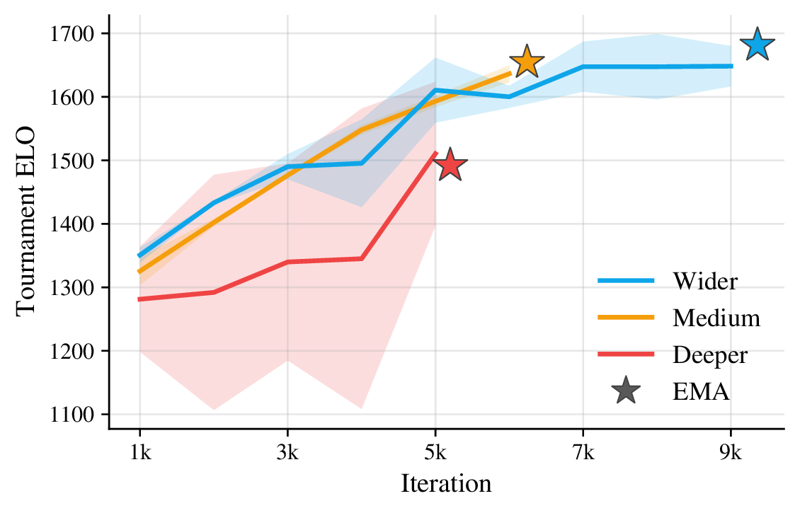
The medium configuration was then scaled up to many more parameters, keeping its depth-to-width proportion. That scaled-up network is the one deployed:
| Parameter | Value |
|---|---|
| depth | 7 |
| embed_dim | 448 |
| n_head | 8 |
| ff_factor | 3 |
| patch_size | 3 |
All in, the deployed network is 15.4M parameters. Half that size might well have done as well or better, but this was a single “yolo” run, and it was good enough.
under the hood Slicing the grid ▶
There are no clean plots for this one, but the trend was consistent across runs: smaller patches were more sample-efficient. Slicing into 3×3 rather than 4×4 squares learned noticeably more per game — though the wall-clock advantage was smaller, since finer patches mean more tokens and a heavier forward pass each step.
Patch size is really a compute knob, because attention cost grows with the square of the token count. On a 24×24 board, 2×2 patches give 12×12 = 144 tokens, while 3×3 give only 8×8 = 64 — so the attention alone is roughly 5× more expensive at 2×2. Iteration speed mattered more here (more games per unit of compute), so 3×3 won out over paying for the bigger forward pass.
3×3 was enough to reach superhuman play, so that's where it stayed. But the sample-efficiency trend points the other way: 2×2 could plausibly be stronger still, for anyone willing to spend the extra compute.
Cherries on top
The remaining pieces were ablated to see which actually matter; a few of them below.
Reward shaping
Round one used potential-based reward shaping, and it helped — probably because, from the supervised checkpoint, RL rushed toward a hyper-aggressive style, and shaping steered the agent toward material advantage. Throughput was also ~100× lower, so a denser reward got more out of each game.
Round two flipped that. With far more data, the win/loss signal alone tells the agent enough about what wins to make shaping unnecessary — and any shaping not completely aligned with winning only biases it towards suboptimal behavior. In the ablation, shaped reward improves slower early, then degrades and destabilizes.
Parameter EMA
At deployment, the network's weights are an exponential moving average of the training iterates rather than the latest checkpoint. The agent is strong without it, but even across 7 days of training on 4×H200s, the EMA checkpoint kept a higher Elo than the last iterate (about 30 Elo by the end of the run). For a one-line change costing essentially zero compute, that's a nice improvement.

Advantage filtering
Many games are decided long before they end — positions where a person would already resign, but the agents play on anyway. If the game then ends as expected, those late samples carry little new information, so there's little point training on them.
So training updates keep only the top 25% of observation–action pairs, ranked by predicted advantage, and drop the rest — which also makes the update step much faster. The trick comes from Sokota et al.'s Stratego work13, where keeping only the highest-advantage transitions saved a lot of wall-clock and was more sample-efficient; it helped here too.
This was ablated on a smaller version of the game, on a single GPU. A smaller fraction gives higher variance across seeds, but also the best single seed. Not every setting was run at full scale, but on the 4-GPU runs the top 25% worked very well.

Hyperparameters
For the tuners: the main hyperparameters, their values, and — more usefully — how much getting each one right seems to matter.
| Hyperparameter | Value | Importance |
|---|---|---|
| ▶Learning rate | clip(0.5·(t+1)-1.1, 5e‑6, 1e‑4) | high |
| Because the 0.5·(t+1)-1.1 term starts well above the cap, the rate stays flat at 1e-4 for the first ~2,000 iterations, then decays as a power law down to the 5e-6 floor. The exact curve barely mattered — power-law and linear decays landed in the same place; what mattered was the range (annealing roughly 1e-4 to 1e-5 was safe). | ||
| ▶Entropy coefficient | 0.05·(t+1)-0.2 | medium |
| In the literature the entropy coefficient is a big knob; here it showed less impact. Across a range of schedules and coefficients, the policy's action-distribution entropy behaved the same way: a sharp drop to ~1 early in training, then a very slow decline, regardless of the schedule. | ||
| ▶Advantage top-fraction | 25% | high |
| See the filtering section above. Beyond stronger agents overall, it sped up iteration: each training run took less wall-clock, leaving room to try more ideas. | ||
| ▶Discount γ | 1.0 | high |
| Keeping γ = 1.0 matters more than it looks. A smaller γ makes learning easier but distorts play, because the timing of the ±1 reward starts to matter. When losing, a discounted agent stalls to delay the −1 and shrink its punishment, instead of gambling on a comeback; when winning, it rushes to bank the +1 sooner, taking risks that hand the opponent counterplay. At γ = 1 the reward is worth the same whenever it lands, so the agent keeps fighting from lost positions and closes out won ones safely. | ||
| ▶GAE λ | 0.9 | high |
| Sokota's Stratego work13 uses λ = 0.5, but higher was better here. In two long-running experiments, λ = 0.7 was ahead for the first 70 hours of training; after that the λ = 0.9 run became stronger and slowly extended its lead. So λ seems to depend not only on the variance of the environment but also on how long you train, i.e. how much data you collect. | ||
| ▶PPO clip ε | 0.2 | low |
| Left at the default, untouched. Conceptually it may play a similar role to the coefficient on the KL term in MMD — both bound how far a single update can move the policy. | ||
| ▶PPO epochs | 1 | medium |
| The default: one pass over each rollout. | ||
| ▶Value-loss coef | 0.5 | medium |
| Weight on the value loss relative to the policy loss. A value of 1.0 was also tried, but it completely broke training, so the default 0.5 stayed. | ||
| ▶Grad-norm clip | 0.267 | low |
| Global gradient-norm clip; the oddly specific 0.267 is taken from Sokota et al.13 | ||
| ▶Parallel environments | 512 | medium |
| The largest number that still bought throughput from adding more; past it the GPUs were saturated. | ||
| ▶Steps per iteration | 512 | medium |
| At some point this switched from 1024 environments × 256 steps to 512 × 512 — the same ~262k transitions per iteration (the advantage filter keeps ~65k), just reshaped into a longer horizon. The intuition: a longer horizon gives less biased advantages, since more of each rollout reaches the true ±1 outcome and leans on the critic's bootstrap less. It seemed to help, though it wasn't ablated. | ||
| ▶Minibatch size | 1024 | medium |
| Minibatch for each gradient step. Not experimented with much. | ||
| ▶Value head (HL-Gauss) | 128 bins, σ 0.04 | medium |
| Categorical value head (HL-Gauss) over [−1, 1] instead of scalar regression. Default parameters. | ||
| ▶EMA decay τ | 0.999 | low |
| Default value, left untouched. See the EMA section. | ||
Honestly, there are too many hyperparameters to ablate properly, and most of the values above are educated guesses or defaults from the literature. The ones that got real attention were the network architecture, then the learning rate and GAE λ. In hindsight, minibatch size deserved more experimentation — left near a default here, it keeps turning up as a surprisingly important factor across RL work, and it's the first thing worth tuning harder next time.
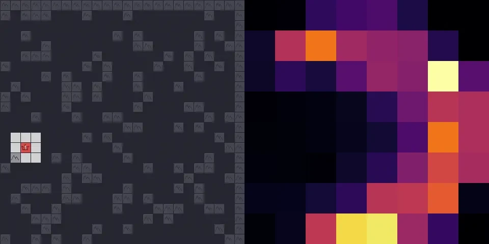
A head that learned to see through the fog
Most of the network is distributed mush under a microscope, but one attention head (value token attending board patches, layer 6, head 4) turns out to encode a belief over where the enemy general is hiding — and it reasons about it very well. It is strikingly accurate, often pinpointing the hidden enemy base within a handful of moves.


under the hood How this head was found ▶
Nothing clever. The value token is the most special token in the sequence, so it serves as the source of the attention queries; their dot product with the keys of every board patch reads off as a heatmap — which patches the value token attends to most.
Then the whole grid of heads (every layer × every attention head) gets laid out, and stepping through games one move at a time reveals the maps. This general-tracking head jumped out immediately. Three or four others looked interpretable too, though their meaning was harder to pin down.
A few heads seemed to switch jobs partway through a game, as if flipped by some event. One that spent the early game tracking castles changed behavior completely the first time the enemy general was revealed — from then on it attended to something else entirely.
Top of the ladder
The agent was evaluated on the public 1v1 ladder. In its first
thousand rated games, played under a few plain nicknames
(Average Joe
among them), it won 815 and
finished as the highest-rated player on the leaderboard —
above every human and every other bot.
zero v3 (74). That
17-point lead over the top human is the same as the gap
between the top human and the player ranked 25th; the top-100
cutoff is 68.
At the time of writing, the highest-ranked human on the live
ladder is shimatetsu at 101, while
Average Joe sits at 118.
A leaderboard rating averages over the whole population, so the head-to-head records against individual top humans are worth a separate look. Each was a normal rated game from the matchmaker, not an exhibition, and both players knew the opponent was a bot.
| Opponent | W | L | Win rate |
|---|---|---|---|
| shimatetsu rank-1 human | 27 | 12 | 69.2% |
| Mithraaaa rank-2 human | 172 | 58 | 74.8% |
| Human.exe best classical bot | 20 | 0 | 100% |
| zero v3 round-one agent | 20 | 0 | 100% |
| Total | 239 | 70 | 77.3% |
Against the two highest-ranked humans alone the agent went
199–70 across 269 games — significant at
p < 0.001 against a coin flip. And the two
bots that mattered, Human.exe and its own
round-one predecessor, were swept 40–0.
The agent in action
“Its ability to flow army in complex situations is phenomenal.”
Human.exe
A few replays of the agent playing, each
picked to show a specific behavior. Swipe through the gallery.
More games can be watched on the agent's ladder accounts,
Average Joe
and
L_7d_gae90_30k_ema.
Closing remarks
At heart, this project is one more case of the bitter lesson paying off, another instance of letting compute go brr :D The jumps didn't come from clever heuristics but from tools that turn raw computation into progress: a simulator fast enough to flood the agent with experience, and an architecture and training loop that keep improving the more you feed them. With those in place, reaching superhuman play took nothing exotic, just general policy-gradient methods and enough experience to learn from, with no game-specific solver and no handcrafted strategy. It still isn't the best bot the recipe could produce. Training the memory rather than hand-crafting it, trading network size for more games played, or giving the agent an explicit belief model over the enemy's army and general's location would all likely help.
To be clear about the order of events: this was the first agent to play this game at a superhuman level. The simulator and the agent were both published before this post went out, and the gap is already closing — people are building on both, some catching up, some arguably ahead, and as of writing the agent sits second on the ladder rather than first. That was always the point of open-sourcing it.
Mostly, the hope is that this is useful to someone. It tries to show the process and not only the final numbers — the dead ends, the patches, the calls worth making differently — because that is the part that rarely survives into a paper, and it's the part most likely to help another applied-RL practitioner shipping something of their own.
Shoutout to Martin for supervising the thesis,
Jonas
for hyping me up through the whole project and giving useful feedback,
EklipZ
for building Human.exe in the first place — beating it
was the whole point of the project, so without it none of this would
exist — and for help getting connected to the real servers and a
lot of useful Generals.io detail, and
Juraj
for implementing the remote connection.
- Generals.io. generals.io
- EklipZ. Human.exe (generals-bot). github.com/EklipZgit/generals-bot
- R. Sutton. The Bitter Lesson. 2019. incompleteideas.net
- J. Perolat et al. Mastering the game of Stratego with model-free multiagent reinforcement learning. Science, 2022. arXiv:2206.15378
- J. Schulman et al. Proximal Policy Optimization Algorithms. 2017. arXiv:1707.06347
- J. Schulman et al. High-Dimensional Continuous Control Using Generalized Advantage Estimation. 2015. arXiv:1506.02438
- A. Ng, D. Harada, S. Russell. Policy Invariance Under Reward Transformations: Theory and Application to Reward Shaping. ICML, 1999. PDF
- G. W. Brown. Iterative Solution of Games by Fictitious Play. Activity Analysis of Production and Allocation, 1951.
- M. Lanctot et al. A Unified Game-Theoretic Approach to Multiagent Reinforcement Learning. NeurIPS, 2017. arXiv:1711.00832
- S. Sokota et al. A Unified Approach to Reinforcement Learning, Quantal Response Equilibria, and Two-Player Zero-Sum Games. ICLR, 2023. arXiv:2206.05825
- M. Rudolph et al. Reevaluating Policy Gradient Methods for Imperfect-Information Games. 2025. arXiv:2502.08938
- J. Heinrich, D. Silver. Deep Reinforcement Learning from Self-Play in Imperfect-Information Games. 2016. arXiv:1603.01121
- S. Sokota et al. Superhuman AI for Stratego Using Self-Play Reinforcement Learning and Test-Time Search. 2025. arXiv:2511.07312
- M. Zinkevich, M. Johanson, M. Bowling, C. Piccione. Regret Minimization in Games with Incomplete Information. NeurIPS, 2007.
If this was useful in your own work, you can cite the round-two paper:
@misc{straka2026generals,
  title         = {Superhuman AI for Generals.io Using Self-Play Reinforcement Learning},
  author        = {Matej Straka and Viliam Lisý and Martin Schmid},
  year          = {2026},
  eprint        = {2606.23348},
  archivePrefix = {arXiv},
  primaryClass  = {cs.LG},
  url           = {https://arxiv.org/abs/2606.23348},
}
